Table of Contents
In which I spare you an abundance of "map"-related puns while explaining what Mean Average Precision is.
(Ok there's one pun.) Since you're reading this you've probably just encountered the term "Mean Average Precision", or MAP. This is a very popular evaluation metric for algorithms that do information retrieval, like google search. If you have an algorithm that is returning a ranked ordering of items, each item is either hit or miss (like relevant vs. irrelevant search results) and items further down in the list are less likely to be used (like search results at the bottom of the page), then maybe MAP is the metric for you!
MAP for Recommender Algorithms
It happens that MAP is also useful for user recommendation systems, like when Amazon shows you a short list of products it thinks you might also want to purchase after you've added something to your cart. Using MAP to evaluate a recommender algorithm implies that you are treating the recommendation like a ranking task. This often makes perfect sense! A user has a finite amount of time and attention, so we want to know not just five products they might like, but also which are most liked or which we are most confident of. This lets you show the top recommendations first and maybe market them more aggressively.
For this kind of task we want a metric that rewards us for getting lots of "correct" or relevant recommendations, and rewards us for having them earlier on in the list (higher ranked). Before we can construct this metric though, we need Precision and Recall. (That's what I call my left and right fist.)
Precision and Recall of a Binary Classifier
I conveniently just learned about these terms in Andrew Ng's ML course on Coursera, so let's start there. If we have binary classifier for predicting having a condition ($y=1$) vs not, then we define:
\begin{align*} \textrm{precision:} \qquad P = \frac{\textrm{# correct positive}}{\textrm{# predicted positive}}\\ \\ \textrm{recall:} \qquad r = \frac{\textrm{# correct positive}}{\textrm{# with condition}} \end{align*}In maybe more familiar terminology, precision is (1 - false positive rate), and the recall is (1 - false negative rate). Actually I'm baffled as to why two new terms were needed for this.
Precision and Recall of Recommender Systems
OK so how does this map (ding!) to recommender systems? In modeling pretty much all recommendation systems we're going to have the following quantities with their corresponding ones in the binary classifier:
| Terminology in Binary Classifier | Terminology in Recommender System |
|---|---|
| # with condition | # of all the possible relevant ("correct") items for a user |
| # predicted positive | # of items we recommended (we predict these items as "relevant") |
| # correct positives | # of our recommendations that are relevant |
OK so now with almost no effort we have:
\begin{align*} \textrm{recommender system precision:} \qquad P = \frac{\textrm{# of our recommendations that are relevant}}{\textrm{# of items we recommended}}\\ \\ \textrm{recommender system recall:} \qquad r = \frac{\textrm{# of our recommendations that are relevant}}{\textrm{# of all the possible relevant items}} \end{align*}Let's say I am asked to recommend $N=5$ products (this means I predict "positive" for five products), from all the possible products there are only $m=3$ that are actually relevant to the user, and my successes and failures in my ranked list are $[0, 1, 1, 0, 0]$. Then:
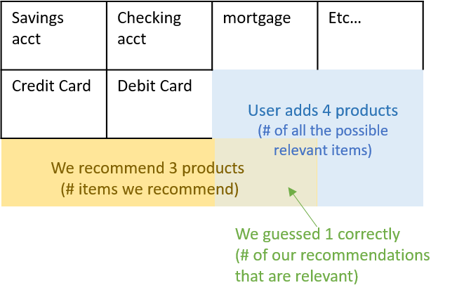
- # of items we recommended = 5
- # of our recommendations that are relevant = 2
- # of all the possible relevant items = 3
- precision = 2/5
- recall = 2/3
Here's a visual example: we're being asked to recommend financial "products" to Bank users and we compare our recommendations to the products that a user actually added the following month (those are all the possible "relevant" ones).
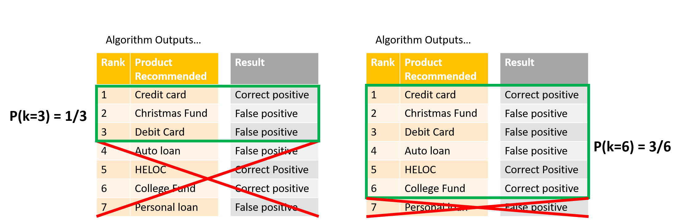
Precision and Recall at Cutoff k
So that's nice, but Precision and Recall don't seem to care about ordering. So instead let's talk about precision and recall at cutoff k. Imagine taking your list of $N$ recommendations and considering only the first element, then only the first two, then only the first three, etc... these subsets can be indexed by $k$. Precision and Recall at cutoff k, $P(k)$ and $r(k)$, are simply the precision and recall calculated by considering only the subset of your recommendations from rank 1 through $k$. Really it would be more intuitive to say "up to cutoff k" rather than "at".
Sticking with the bank example, here is what I mean:
Average Precision
OK are you ready for Average Precision now? If we are asked to recommend $N$ items, the number of relevant items in the full space of items is $m$, then:
\begin{align*} \textrm{AP@N} = \frac{1}{m}\sum_{k=1}^N \textrm{($P(k)$ if $k^{th}$ item was relevant)} = \frac{1}{m}\sum_{k=1}^N P(k)\cdot rel(k), \end{align*}where $rel(k)$ is just an indicator that says whether that $k^{th}$ item was relevant ($rel(k)=1$) or not ($rel(k)=0$). I'd like to point out that instead of recommending $N$ items would could have recommended, say, $2N$, but the AP@N metric says we only care about the average precision up to the $N^{th}$ item.
Examples and Intuition for AP
Let's imagine recommending $N=3$ products (AP@3) to a user who actually added a total of $m=3$ products. Here are some examples of outcomes for our algorithm:
| __Recommendations__ | __Precision @k's__ | __AP@3__ |
|---|---|---|
| [0, 0, 1] | [0, 0, 1/3] | (1/3)(1/3) = 0.11 |
| [0, 1, 1] | [0, 1/2, 2/3] | (1/3)[(1/2) + (2/3)] = 0.38 |
| [1, 1, 1] | [1/1, 2/2, 3/3] | (1/3)[(1) + (2/2) + (3/3)] = 1 |
First notice that the more correct recommendations I have, the larger my AP. This is because the $k^{th}$ subset precision is included in AP sum only if you got the $k^{th}$ recommendation correct, thus AP rewards you for giving correct recommendations (surprising absolutely no one).
There is more subtletly here though! In each row I've bolded the $P(k)$ term which came from the correct recommendation in the third slot. Notice it is larger when there have been more successes in front of it - that's because the precision of the $k^{th}$ subset is higher the more correct guesses you've had up to point $k$. Thus, AP rewards you for front-loading the recommendations that are most likely to be correct.
These two features are what makes AP a useful metric when your algorithm is returning a ranked ordering of items where each item is either correct or incorrect, and items further down in the list are less likely to be used. One more set of examples might make this second point a little clearer.
| __Recommendations__ | __Precision @k's__ | __AP@3__ |
|---|---|---|
| [1, 0, 0] | [1/1, 1/2, 1/3] | (1/3)(1) = 0.33 |
| [0, 1, 0] | [0, 1/2, 1/3] | (1/3)(1/2) = 0.15 |
| [0, 0, 1] | [0, 0, 1/3] | (1/3)(1/3) = 0.11 |
In all these cases you got just one recommendations correct, but AP was higher the further up the ranking that correct guess fell.
A final point of note is that adding another recommendation can never decrease your AP score, so if you are asked for $N$ recommendations give all of them, even if you don't feel very confident about the ones lower down the list! AP will never penalize you for tacking on additional recommendations to your list - just make sure you front-load the best ones.
The "Mean" in MAP
OK that was Average Precision, which applies to a single data point (like a single user). What about MAP@N? All that remains is to average the AP@N metric over all your $|U|$ users. Yes, an average of an average.
\begin{align*} \textrm{MAP@N} = \frac{1}{|U|}\sum_{u=1}^|U|(\textrm{AP@N})_u = \frac{1}{|U|} \sum_{u=1}^|U| \frac{1}{m}\sum_{k=1}^N P_u(k)\cdot rel_u(k). \end{align*}Common Variations on AP Formula
Often you see the AP metric modified slightly when there might be more possible correct recommendations then the number of recommendations you are asked to give. Say, a super active user at the bank who adds $m=10$ accounts the next month, while your algorithm is only supposed to report $N=5$. In this case the normalization factor used is $1/\textrm{min}(m, N)$, which prevents your AP score from being unfairly suppressed when your number of recommendations couldn't possibly capture all the correct ones.
\begin{align*} \textrm{AP@N} = \frac{1}{\textrm{min}(m,N)}\sum_{k=1}^N P(k)\cdot rel(k). \end{align*}You also might encounter a somewhat sloppier usage where there is no indicator function $rel(k)$ in the AP@N sum. In this case the precision at cutoff $k$ is being implictly defined to be zero when the $k^{th}$ recommendation was incorrect, that way it still doesn't contribute to the sum:
\begin{align*} \textrm{AP@N} = \frac{1}{m}\sum_{k=1}^N P(k),\\ P(k) = 0 \textrm{ if $k^{th}$ element is irrelevant / incorrect.} \end{align*}Finally, if it's possible for there to be no relevant or correct recommendations possible ($m=0$) then often the AP is defined to be zero for those points. Note that it will have the effect of dragging the MAP number of an algorithm down the more users there are who didn't actually add any products. This doesn't matter for comparing the performance of two algorithms on the same data set, but it does mean that you shouldn't place any kind of absolute meaning on the final number.
\begin{align*} \textrm{AP@N} = \frac{1}{\textrm{min}(m,N)}\sum_{k=1}^N P(k)\cdot rel(k) \qquad \textrm{ if $m\neq 0$,}\\ AP = 0 \qquad \textrm{if $m=0$}. \end{align*}So Why Did I Bother Defining Recall?
There is an alternative formulation for the AP in terms of Precision and Recall, and I didn't want you to feel left out when people start talking about it at parties:
\begin{align*} \textrm{AP@N} = \sum_{k=1}^N \textrm{(precision at $k$)}\cdot\textrm{(change in recall at $k$)} = \sum_{k=1}^N P(k)\Delta r(k), \end{align*}where $\Delta r(k)$ is the change in recall from the $k-1^{th}$ to the $k^{th}$ subset. This formulation is actually kind of nice because we don't need to "leave out" terms in the sum with an indicator function, instead the change in recall term is zero when the $k^{th}$ recommendation is incorrect so those guys get wiped out anyway. Hopefully you noticed that the prefactor $1/m$ is missing too, it turns out that when the $k^{th}$ recommendation is correct the change in recall is exactly $1/m$. OK let me stop talking and make with the examples. Same as before, recommending $N=3$ products (AP@3) to a user who actually added a total of $m=3$ products:
| __Recs__ | __Prec @k's__ | __Recall @k's__ | __Change r @k's__ | __AP@3__ |
|---|---|---|---|---|
| [0, 0, 1] | [0, 0, 1/3] | [0, 0, 1/3] | [0, 0, 1/3] | (1/3)(1/3) = 0.11 |
| [0, 1, 1] | [0, 1/2, 2/3] | [0, 1/3, 2/3] | [0, 1/3, 1/3] | (1/3)(1/2) + (1/3)(2/3) = 0.38 |
| [1, 1, 1] | [1, 2/2, 3/3] | [1/3, 2/3, 3/3] | [1/3, 1/3, 1/3] | (1/3)(1) + (1/3)(1) + (1/3)(1) = 1 |
| __Recs__ | __Prec @k's__ | __Recall @k's__ | __Change r @k's__ | __AP@3__ |
|---|---|---|---|---|
| [1, 0, 0] | [1, 1/2, 1/3] | [1/3, 1/3, 1/3] | [1/3, 0, 0] | (1)(1/3) = 0.33 |
| [0, 1, 0] | [0, 1/2, 1/3] | [0, 1/3, 1/3] | [0, 1/3, 0] | (1/2)(1/3) = 0.15 |
| [0, 0, 1] | [0, 0, 1/3] | [0, 0, 1/3] | [0, 0, 1/3] | (1/3)(1/3) = 0.11 |
Hopefully you can convince yourself that you are getting exactly the same result for this formulation of AP as we got before.
Graphical Representation of $P(i)$ and $r(i)$
We can think of $P(i)$ and $r(i)$ as functions of the index $i$, and we can plot them accordingly, e.g. $P(i)$ vs. $i$. The resulting plot would of course depend heavily on the particular sequence of correct/incorrect recommendations that we are indexing through. More often what you see is a plot in the $P(i)$ x $r(i)$ plane that traces out the trajectory of both these quantities as you index through the list of recommendations. Analytically we can already imagine what such a trajectory will do: if at the next $i$ we got a correct recommendation then both precision and recall should increase, whereas if we got that recommendation wrong then precision will decrease while recall will be unchanged.
Let me show you :)
recoms = [0, 1, 0, 1, 0, 1, 1]  # N = 7
NUM_ACTUAL_ADDED_ACCT = 5
precs = []
recalls = []

for indx, rec in enumerate(recoms):
    precs.append(sum(recoms[:indx+1])/(indx+1))
    recalls.append(sum(recoms[:indx+1])/NUM_ACTUAL_ADDED_ACCT)

print(precs)
print(recalls)
import matplotlib.pyplot as plt
% matplotlib inline
fig, ax = plt.subplots()
ax.plot(recalls, precs, markersize=10, marker="o")
ax.set_xlabel("Recall")
ax.set_ylabel("Precision")
ax.set_title("P(i) vs. r(i) for Increasing $i$ for AP@7")

The jaggedness of this type of plot has lead to the creation of some "smoothed" or "interpolated" average precision metrics as alternatives, but I'll not talk about them here.
To Summarize...
MAP is very popular evaluation metric for algorithms that do information retrieval like google search results, but it also can apply to user-targeted product recommendations. If you have an algorithm that is returning a ranked ordering of items, each item is either hit or miss (like relevant vs. irrelevant search results) and items further down in the list are less likely to be used/seen (like search results at the bottom of the page), then MAP might be a useful metric.
Using MAP to evaluate a recommender algorithm implies that you are treating the recommendation like a ranking task. This often makes perfect sense since a user has a finite amount of time and attention and we want to show the top recommendations first and maybe market them more aggressively.
In recommendation systems MAP computes the mean of the Average Precision (AP) over all your users. The AP is a measure that takes in a ranked list of your $N$ recommendations and compares it to a list of the true set of "correct" or "relevant" recommendations for that user. AP rewards you for having a lot of "correct" (relevant) recommendations in your list, and rewards you for putting the most likely correct recommendations at the top (you are penalized more when incorrect guesses are higher up in the ranking). So order of "hits" and "misses" matters a lot in computing an AP score, but once you have front-loaded your best guesses you can never decrease your AP by tacking on more.
Further Reading on MAP
- from the source itself... wikipedia
- from an all-things-ML blog fast ML
- from Stanford class slides
- from a DS blog
- from a Stanford online book
- from June Andrews on why MAP is "mean"
- from Cornell class slides